Diffusion Models

Introduction

Diffusion models are a class of generative models that learn to create data (images, audio, video, molecules, etc.) by reversing a gradual noising process. They belong to the family of likelihood-based models and have surpassed GANs on many benchmarks.

Model Family	Sampling Speed	Sample Quality	Training Stability
GAN	⚡ Fast	⭐⭐⭐	❌ Unstable
VAE	⚡ Fast	⭐⭐	✅ Stable
Flow	Medium	⭐⭐⭐	✅ Stable
Diffusion	🐢 Slow*	⭐⭐⭐⭐	✅ Very Stable

DDIM, consistency models, and latent diffusion significantly speed up sampling.

Core Intuition

Think of a sand castle on a beach:

Forward process: Waves (noise) gradually erode the castle until nothing remains but flat sand (pure Gaussian noise).
Reverse process: A model learns how to rebuild the castle from noisy sand — one denoising step at a time.

The key insight is that if you can reverse small noising steps, you can generate complex data from pure noise.

x₀ (clean image)
  → x₁ (tiny noise added)
    → x₂ (more noise)
      → ...
        → xT ≈ N(0, I)   ← pure Gaussian noise

Reverse: xT → x_{T-1} → ... → x₁ → x₀  (learned by neural network)

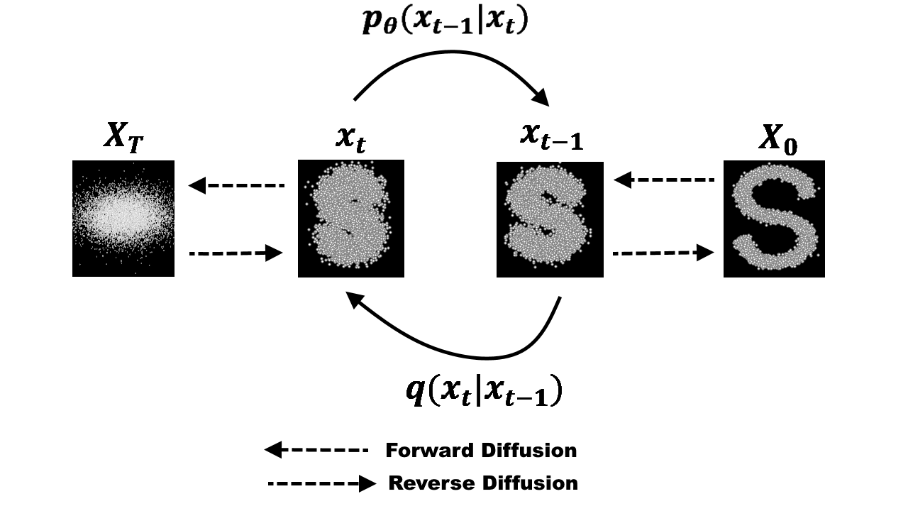Forward and Reverse Process

The Forward Process (Noising)

Given a data sample $x_0 \sim q(x_0)$ , the forward process adds Gaussian noise over $T$ timesteps:

q(x_t \mid x_{t-1}) = \mathcal{N}\Big(x_t \,;\, \sqrt{1 - \beta_t}\, x_{t-1},\; \beta_t \mathbf{I}\Big)

Where:

$\beta_t \in (0, 1)$ is the noise schedule at step $t$ (e.g., linear, cosine)
$\mathcal{N}(\mu, \sigma^2 \mathbf{I})$ denotes a Gaussian with mean $\mu$ and variance $\sigma^2 \mathbf{I}$
$T$ is typically 1000 steps

#Closed-Form Marginal

Define $\alpha_t = 1 - \beta_t$ and $\bar{\alpha}_t = \prod_{s=1}^{t} \alpha_s$ (cumulative product). Then:

q(x_t \mid x_0) = \mathcal{N}\Big(x_t \,;\, \sqrt{\bar{\alpha}_t}\, x_0,\; (1 - \bar{\alpha}_t)\, \mathbf{I}\Big)

This allows directly sampling $x_t$ at any timestep without iterating through all previous steps:

x_t = \sqrt{\bar{\alpha}_t}\, x_0 + \sqrt{1 - \bar{\alpha}_t}\, \varepsilon \quad \text{where} \quad \varepsilon \sim \mathcal{N}(0, \mathbf{I})

#Noise Schedules

import numpy as np
 
T = 1000
 
# Linear schedule (Ho et al. 2020)
beta_linear = np.linspace(1e-4, 0.02, T)
 
# Cosine schedule (Nichol & Dhariwal 2021) — better for images
def cosine_schedule(T, s=0.008):
    t = np.linspace(0, T, T + 1)
    f = np.cos(((t / T + s) / (1 + s)) * np.pi / 2) ** 2
    alphas_bar = f / f[0]
    betas = 1 - alphas_bar[1:] / alphas_bar[:-1]
    return np.clip(betas, 0, 0.999)
 
beta_cosine = cosine_schedule(T)

Denoising

The reverse process is also Gaussian (for small $\beta_t$ ):

p_\theta(x_{t-1} \mid x_t) = \mathcal{N}\Big(x_{t-1} \,;\, \mu_\theta(x_t, t),\; \Sigma_\theta(x_t, t)\Big)

The neural network (typically a U-Net) predicts either:

The noise $\varepsilon_\theta(x_t, t)$ — DDPM parameterization
The clean image $\hat{x}_0$ — x-prediction parameterization
The score $\nabla_{x_t} \log q(x_t)$ — score-based view

#Computing the Posterior Mean

Given the noise prediction $\varepsilon_\theta$ , the posterior mean is:

\mu_\theta(x_t, t) = \frac{1}{\sqrt{\alpha_t}} \left[ x_t - \frac{\beta_t}{\sqrt{1 - \bar{\alpha}_t}} \, \varepsilon_\theta(x_t, t) \right]

#Sampling Step (DDPM)

def ddpm_sample_step(model, x_t, t, alpha_bar, alpha_bar_prev, beta_t):
    # Predict noise
    eps_pred = model(x_t, t)
 
    # Compute predicted clean image
    x0_pred = (x_t - (1 - alpha_bar)**0.5 * eps_pred) / alpha_bar**0.5
 
    # Compute posterior mean
    mu = (1 / (1 - beta_t)**0.5) * (
        x_t - beta_t / (1 - alpha_bar)**0.5 * eps_pred
    )
 
    # Add noise (except at t=0)
    sigma = beta_t**0.5
    z = torch.randn_like(x_t) if t > 0 else 0
    x_prev = mu + sigma * z
    return x_prev

Training Objective

#Variational Lower Bound (ELBO)

The model maximizes the evidence lower bound:

L = \mathbb{E}_q \left[ \log p(x_T) + \sum_t \log p(x_{t-1} \mid x_t) - \log q(x_t \mid x_{t-1}) \right]

This decomposes into KL-divergence terms. Ho et al. (2020) showed this simplifies to the form below.

#Simplified Loss (DDPM)

L_{\text{simple}} = \mathbb{E}_{t, x_0, \varepsilon} \left[ \left\| \varepsilon - \varepsilon_\theta\Big( \sqrt{\bar{\alpha}_t}\, x_0 + \sqrt{1 - \bar{\alpha}_t}\, \varepsilon,\; t \Big) \right\|^2 \right]

In plain English: predict the noise $\varepsilon$ that was added to the clean image $x_0$ to get $x_t$ .

#Training Loop

import torch
import torch.nn.functional as F
 
def train_step(model, x0, noise_schedule):
    batch_size = x0.shape[0]
 
    # Sample random timesteps
    t = torch.randint(0, T, (batch_size,), device=x0.device)
 
    # Sample noise
    epsilon = torch.randn_like(x0)
 
    # Create noisy image: xₜ = √ᾱₜ · x₀ + √(1−ᾱₜ) · ε
    alpha_bar_t = noise_schedule.alpha_bar[t].view(-1, 1, 1, 1)
    x_t = alpha_bar_t.sqrt() * x0 + (1 - alpha_bar_t).sqrt() * epsilon
 
    # Predict noise
    epsilon_pred = model(x_t, t)
 
    # Simple MSE loss
    loss = F.mse_loss(epsilon_pred, epsilon)
    return loss

Score Matching & DDPM

#Score Functions

The score function is the gradient of the log-density:

s(x) = \nabla_x \log p(x)

For a noisy distribution $q(x_t \mid x_0)$ , the score is:

\nabla_{x_t} \log q(x_t \mid x_0) = - \frac{\varepsilon}{\sqrt{1 - \bar{\alpha}_t}}

#Connection to Noise Prediction

So predicting the noise is equivalent to predicting (a scaled) score:

\varepsilon_\theta(x_t, t) \approx - \sqrt{1 - \bar{\alpha}_t} \, \nabla_{x_t} \log q(x_t)

This connects DDPM to score-based generative models (Song & Ermon, 2019).

DDIM: Faster Sampling

DDPM requires T = 1000 steps. DDIM (Denoising Diffusion Implicit Models, Song et al. 2020) achieves similar quality in 10–50 steps by using a non-Markovian update.

#DDIM Update Rule

x_{t-1} = \sqrt{\bar{\alpha}_{t-1}} \, \hat{x}_0(x_t) + \sqrt{1 - \bar{\alpha}_{t-1} - \sigma_t^2} \, \varepsilon_\theta(x_t, t) + \sigma_t \, \varepsilon

Where:

$\hat{x}_0(x_t) = \dfrac{x_t - \sqrt{1 - \bar{\alpha}_t}\, \varepsilon_\theta(x_t, t)}{\sqrt{\bar{\alpha}_t}}$ is the predicted clean image
$\sigma_t = \eta \, \sqrt{\dfrac{1 - \bar{\alpha}_{t-1}}{1 - \bar{\alpha}_t}} \, \sqrt{1 - \alpha_t}$ controls stochasticity
When $\eta = 0$ : fully deterministic (same noise → same image)
When $\eta = 1$ : reduces to DDPM

#Speedup Comparison

Sampler	Steps	FID (CIFAR-10)	Time
DDPM	1000	3.17	~20 min
DDIM (η=0)	50	4.16	~1 min
DDIM (η=0)	10	6.84	~12 sec

Conditional Diffusion (Guided Generation)

To condition generation on a label y (text, class, image), we modify the reverse process.

#Classifier Guidance

(Dhariwal & Nichol, 2021)

Use a classifier $p_\phi(y \mid x_t)$ to steer sampling:

\nabla_{x_t} \log p(x_t \mid y) = \nabla_{x_t} \log p(x_t) + \gamma \, \nabla_{x_t} \log p_\phi(y \mid x_t)

Where γ is the guidance scale (higher = more condition-faithful but less diverse).

#Classifier-Free Guidance (CFG)

(Ho & Salimans, 2022)

No external classifier needed. Train with random conditioning dropout:

# During training: randomly drop condition
if random.random() < dropout_prob:
    condition = null_token  # unconditional
 
# During inference: interpolate conditional and unconditional predictions
eps_pred = eps_uncond + guidance_scale * (eps_cond - eps_uncond)

Effective score:

\tilde{\varepsilon}_\theta(x_t, y) = \varepsilon_\theta(x_t, \varnothing) + \gamma \left[ \varepsilon_\theta(x_t, y) - \varepsilon_\theta(x_t, \varnothing) \right]

This is the backbone of Stable Diffusion, DALL·E 2, and Imagen.

Example

Task: Generate a 4×4 Grayscale Image from Noise

Setup: $T = 4$ , linear $\beta$ schedule: $\beta = [0.1, 0.2, 0.3, 0.4]$

\alpha_t = 1 - \beta_t = [0.90, 0.80, 0.70, 0.60]

\bar{\alpha}_t = \operatorname{cumprod}(\alpha_t) = [0.90, 0.72, 0.504, 0.302]

#Step 1 — Forward (Add Noise to Clean Image $x_0$ )

x_0 = \begin{bmatrix} 0.8 & 0.2 \\ 0.5 & 0.9 \end{bmatrix}

\varepsilon \sim \mathcal{N}(0, \mathbf{I}) = \begin{bmatrix} 0.3 & -0.1 \\ 0.6 & 0.2 \end{bmatrix}

At $t = 2$ : $\bar{\alpha}_2 = 0.72$

x_2 = \sqrt{0.72} \, x_0 + \sqrt{1 - 0.72} \, \varepsilon

= 0.849 \, x_0 + 0.529 \, \varepsilon

= \begin{bmatrix} 0.838 & 0.117 \\ 0.741 & 0.870 \end{bmatrix}

#Step 2 — Reverse Step (Model Predicts ε from x₂)

# Model takes x_t and t, outputs predicted noise
eps_pred = model(x_2, t=2)
# Suppose eps_pred ≈ [[0.29, -0.09], [0.58, 0.19]]  (close to true ε)
 
alpha_2     = 0.80
alpha_bar_2 = 0.72
beta_2      = 0.20
 
coeff = beta_2 / (1 - alpha_bar_2)**0.5   # = 0.20 / 0.529 = 0.378
mu = (1 / alpha_2**0.5) * (x_2 - coeff * eps_pred)
 
# Add noise for stochastic sampling
sigma = beta_2**0.5   # = 0.447
z = sample_from_N(0, I)
x_1 = mu + sigma * z

#Step 3 — Repeat Until x₀

Each reverse step brings the sample closer to a realistic image, guided by what the model learned during training.

Tools & Libraries

#Hugging Face Diffusers (Most Popular)

# pip install diffusers transformers accelerate
 
from diffusers import StableDiffusionPipeline
import torch
 
pipe = StableDiffusionPipeline.from_pretrained(
    "runwayml/stable-diffusion-v1-5",
    torch_dtype=torch.float16
)
pipe = pipe.to("cuda")
 
image = pipe(
    prompt="a cat wearing a wizard hat, digital art",
    num_inference_steps=50,    # DDIM steps
    guidance_scale=7.5,        # classifier-free guidance scale
    height=512,
    width=512,
).images[0]
 
image.save("output.png")

#Stable Diffusion XL

from diffusers import DiffusionPipeline
 
pipe = DiffusionPipeline.from_pretrained(
    "stabilityai/stable-diffusion-xl-base-1.0",
    torch_dtype=torch.float16,
    use_safetensors=True,
    variant="fp16"
)
pipe.to("cuda")
 
image = pipe(
    prompt="astronaut in a jungle, cold color palette"
).images[0]

#Training Your Own (minDiffusion)

import torch
import torch.nn as nn
from torch.optim import Adam
 
class SimpleUNet(nn.Module):
    """Tiny U-Net for educational purposes"""
    def __init__(self, channels=1):
        super().__init__()
        self.enc = nn.Sequential(
            nn.Conv2d(channels + 1, 64, 3, padding=1), nn.ReLU(),
            nn.Conv2d(64, 64, 3, padding=1), nn.ReLU(),
        )
        self.dec = nn.Sequential(
            nn.Conv2d(64, 64, 3, padding=1), nn.ReLU(),
            nn.Conv2d(64, channels, 3, padding=1),
        )
 
    def forward(self, x, t):
        t_map = t.float().view(-1, 1, 1, 1).expand(-1, 1, *x.shape[2:]) / 1000
        x_in = torch.cat([x, t_map], dim=1)
        return self.dec(self.enc(x_in))
 
 
class DDPM:
    def __init__(self, T=1000, beta_start=1e-4, beta_end=0.02):
        self.T = T
        self.betas = torch.linspace(beta_start, beta_end, T)
        self.alphas = 1 - self.betas
        self.alpha_bars = torch.cumprod(self.alphas, dim=0)
 
    def q_sample(self, x0, t, noise=None):
        """Forward process: add noise at timestep t"""
        if noise is None:
            noise = torch.randn_like(x0)
        ab = self.alpha_bars[t].view(-1, 1, 1, 1)
        return ab.sqrt() * x0 + (1 - ab).sqrt() * noise, noise
 
    @torch.no_grad()
    def p_sample(self, model, x, t_idx):
        """One reverse step"""
        t = torch.full((x.shape[0],), t_idx, device=x.device, dtype=torch.long)
        eps = model(x, t)
        alpha     = self.alphas[t_idx]
        alpha_bar = self.alpha_bars[t_idx]
        beta      = self.betas[t_idx]
        mu = (1 / alpha.sqrt()) * (x - beta / (1 - alpha_bar).sqrt() * eps)
        if t_idx > 0:
            z = torch.randn_like(x)
            return mu + beta.sqrt() * z
        return mu
 
    @torch.no_grad()
    def sample(self, model, shape):
        """Full sampling loop"""
        x = torch.randn(shape)
        for t in reversed(range(self.T)):
            x = self.p_sample(model, x, t)
        return x

#Other Key Libraries

Library	Use Case	Link
`diffusers`	Production pipelines (SD, SDXL, …)	huggingface.co/docs/diffusers
`denoising-diffusion-pytorch`	Clean research codebase	github.com/lucidrains
`score_sde`	Score-based models (Song et al.)	github.com/yang-song/score_sde
`k-diffusion`	Advanced samplers (DPM-Solver++)	github.com/crowsonkb
`openai/consistency_models`	Consistency models (1-step)	github.com/openai
`ComfyUI`	Node-based GUI for diffusion	github.com/comfyanonymous/ComfyUI
`AUTOMATIC1111`	Web UI for Stable Diffusion	github.com/AUTOMATIC1111

Summary

Category	Details
Forward Process	$q(x_t \mid x_{t-1}) = \mathcal{N}(\sqrt{1 - \beta_t}\, x_{t-1},\; \beta_t \mathbf{I})$
Closed Form	$x_t = \sqrt{\bar{\alpha}_t}\, x_0 + \sqrt{1 - \bar{\alpha}_t}\, \varepsilon,\;\; \varepsilon \sim \mathcal{N}(0, \mathbf{I})$
Reverse Process	$p_\theta(x_{t-1} \mid x_t) = \mathcal{N}(\mu_\theta(x_t, t),\; \Sigma_\theta(x_t, t))$
Loss	$L = \mathbb{E}\left[\\|\varepsilon - \varepsilon_\theta(\sqrt{\bar{\alpha}_t}\, x_0 + \sqrt{1 - \bar{\alpha}_t}\, \varepsilon,\; t)\\|^2\right]$
DDIM (fast)	Non-Markovian, deterministic when $\eta = 0$
CFG	$\tilde{\varepsilon} = \varepsilon_{\text{uncond}} + \gamma(\varepsilon_{\text{cond}} - \varepsilon_{\text{uncond}})$
Key Papers	DDPM (Ho 2020), DDIM (Song 2020), Improved DDPM (Nichol 2021), LDM / Stable Diffusion (Rombach 2022), Classifier-Free Guidance (Ho 2022)
Architecture	U-Net with sinusoidal time embeddings
Conditioning	Cross-attention for text (CLIP embeddings)
Latent Diffusion	Operates in VAE latent space (≈4× smaller)

#Quick Reference: Hyperparameters

# Typical DDPM config
T: 1000                    # diffusion timesteps
beta_schedule: cosine      # linear or cosine
beta_start: 0.0001
beta_end: 0.02
model: unet
time_embedding: sinusoidal
channels: [128, 256, 512, 1024]
attention_resolutions: [16, 8]
 
# Inference
num_inference_steps: 50    # DDIM
guidance_scale: 7.5        # CFG (1=no guidance, 7-15=typical)
eta: 0.0                   # 0=DDIM deterministic, 1=DDPM stochastic

References: Ho et al. (2020) — DDPM · Song et al. (2020) — DDIM · Nichol & Dhariwal (2021) — Improved DDPM · Rombach et al. (2022) — Latent Diffusion · Ho & Salimans (2022) — CFG